Code
import numpy as np
import matplotlib.pyplot as plt
import sympy as spimport numpy as np
import matplotlib.pyplot as plt
import sympy as spLösen Sie die Differentialgelichung \(\ddot{y} + 3\dot{y} + 2y = 0\) mit den Anfangsbedingungen \(y(0)=2\) und \(\dot{y}(0)= -3\) von Hand und überprüfen Sie Ihr Ergebnis am Computer symbolisch.
Bestimmen Sie die Lösungen folgender GDGL bzw. Anfangswertprobleme. Beschreiben Sie die Lösungen und deren Verhalten für \(x \rightarrow \infty\).
Quelle: Farlow: An Introduction to Differential Equations and their Applications. Sec. 3.4., Example 1, p. 131f.
Wir betrachten die GDGL \(y''(x) - 2y'(x) + y(x) = e^{3x}\).
Quelle: Bronson: Differential Equations. 4. Auflage, Aufgabe 8.23, S. 79.
Bestimmen Sie die Lösungen folgender Anfangswertprobleme und beschreiben Sie die Lösungen und deren Verhalten für \(x \rightarrow \infty\)
Quelle: Dietmaier, p. 474, Aufgaben 12.9 b) und c)
\(y(t) = e^{-t} + e^{-2t}\)
sp.init_printing()

t = sp.symbols('t')
y = sp.symbols('y', cls=sp.Function)
diffeq = sp.Eq(y(t).diff(t).diff(t) + 3*y(t).diff(t) + 2*y(t), 0)
diffeq
\(\displaystyle 2 y{\left(t \right)} + 3 \frac{d}{d t} y{\left(t \right)} + \frac{d^{2}}{d t^{2}} y{\left(t \right)} = 0\)
ys = sp.dsolve(diffeq, y(t))
ys
\(\displaystyle y{\left(t \right)} = \left(C_{1} + C_{2} e^{- t}\right) e^{- t}\)
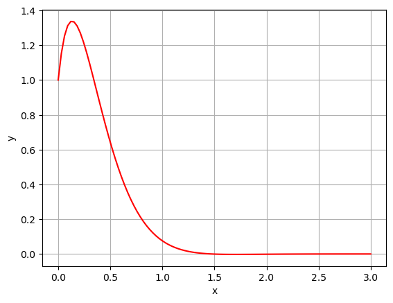
sp.init_printing(False)x = np.linspace(0,3, 100)
y = np.exp(-3*x)*(1 + 5*x)
plt.figure(figsize=(6,3))
plt.plot(x, y,'-r')
plt.xlabel('x')
plt.ylabel('y')
plt.grid(True)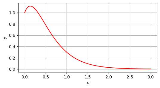
x = np.linspace(0,3, 100)
y = np.exp(-4*x)*(np.cos(2*x) + 5*np.sin(2*x))

plt.figure()
plt.plot(x, y,'-r')
plt.xlabel('x')
plt.ylabel('y')
plt.grid(True)
print(np.min(y))
-0.0024990299146947434