Übung - Mehrdimensionale Funktionen

Code

import numpy as np
import matplotlib.pyplot as plt
import matplotlib.patches as mpl

Code

plt.rcParams['figure.figsize']=(4,4)

Aufgaben

Aufgabe MF1: Kurve und Geschwindigkeit

Sei \(f:\mathbb{R} \rightarrow \mathbb{R}^2\) die Kurve \(f(t)= \begin{pmatrix} x(t) \\ y(t) \end{pmatrix} = \sqrt{t}\begin{pmatrix} \cos(\pi t) \\ \sin(\pi t) \end{pmatrix}\)

1. Erstellen Sie einen Plot der Kurve für \(t\in[0, 2]\).
2. Berechnen Sie den Geschwindigkeitsvektor für jeden Zeitpunkt \(t\) und zeichen Sie mit Hilfe des Befehls quiver Geschwindigkeitsvektoren in Ihren Plot ein. Tipp: Verwenden Sie die scale-Option.
3. Bestimmen und zeichnen Sie Kurve sowie Geschwindigkeitsvektor in Polarkoordinaten.

Aufgabe MF2: Kurve, Tangente

Gegeben ist die Kurve \(\begin{pmatrix} x(t) \\ y(t) \end{pmatrix} = \begin{pmatrix} \sin(2t) \\ \cos(3t) \end{pmatrix}\).

1. Berechnen Sie die Tangente an die Kurve bei \(t=1\).
2. Plotten Sie die Kurve im Bereich \(t\in[-3,3]\) in Python.

Aufgabe MF3: Gradient, Betrag des Gradienten

Gegeben ist das Skalarfeld \(\phi(x,y,z)=10 x^2 y^3 - 5 xyz^2\).

1. Berechnen Sie den Gradienten des Skalarfelds.
2. Berechnen Sie den Betrag des Gradienten im Punkt \(P=(1,-1,2)\).

Aufgabe MF4: Divergenz eines Vektorfelds

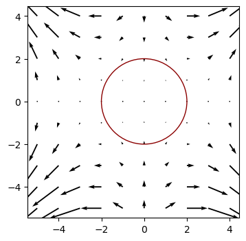
Gegeben ist das Vektorfeld \(\mathbf{F}=\begin{pmatrix} xy^2 \\ x^2y-4y \end{pmatrix}\).

1. In welchen Punkten der x-y Ebene verschwindet die Divergenz des Vektorfelds.
2. Plotten Sie das Vektorfeld sowie die Punkte, in welchen die Divergenz des Vektorfelds verschwindet.

Lösungen

Lösung MF1: Kurve und Geschwindigkeit

1. Siehe Code.
2. Der Geschwindigkeitsvektor zum Zeitpunkt \(t\) ist der Vektor der ersten Ableitungen: \(f'(t)= \begin{pmatrix} x'(t) \\ y'(t) \end{pmatrix} = \begin{pmatrix} \frac{1}{2 \sqrt{t}}\cos(\pi t) - \sqrt{t}\pi\sin(\pi t) \\ \frac{1}{2 \sqrt{t}}\sin(\pi t) + \sqrt{t}\pi\cos(\pi t) \end{pmatrix}\). Siehe Code.
3. \(r(t) = \sqrt{t}\), \(\varphi(t) = \pi t\). \(r'(t) = \frac{1}{2 \sqrt{t}}\), \(\varphi'(t) = \pi\). Siehe Code.

Code

t = np.linspace(0.01, 2)

x = np.sqrt(t)*np.cos(np.pi*t)
y = np.sqrt(t)*np.sin(np.pi*t)

xp = 0.5/np.sqrt(t)*np.cos(np.pi*t) - np.pi*np.sqrt(t)*np.sin(np.pi*t)
yp = 0.5/np.sqrt(t)*np.sin(np.pi*t) + np.pi*np.sqrt(t)*np.cos(np.pi*t)

plt.figure()
plt.plot(x, y, 'r')
plt.quiver(x, y, xp, yp, scale_units='xy', scale= 3)
plt.xlabel('x')
plt.ylabel('y')
plt.xlim(-2, 2)
plt.ylim(-2, 2)
plt.grid(True)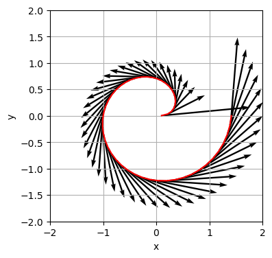

Code

r = np.sqrt(t)
phi = np.pi*t

rp = 0.5/np.sqrt(t)
phip = np.pi*np.ones(r.shape)

Code

plt.figure()
plt.plot(r, phi, 'r')
plt.quiver(r, phi, rp, phip, scale_units='xy', scale= 4)
plt.xlabel('r')
plt.ylabel('phi')
plt.xlim(0, 8)
plt.ylim(0, 8)
plt.grid(True)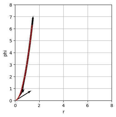

Lösung MF2: Kurve, Tangente

1. Ort bei \(t=1\) ist \(\begin{pmatrix} x(1) \\ y(1) \end{pmatrix} = \begin{pmatrix} \sin(2) \\ \cos(3) \end{pmatrix}\). Geschwindigkeitsvektor bei \(t=1\) ist \(\begin{pmatrix} x'(1) \\ y'(1) \end{pmatrix} = \begin{pmatrix} 2\cos(2) \\ -3\sin(3) \end{pmatrix}\). Tangentengleichung: \(\begin{pmatrix} x_T(t) \\ y_T(t) \end{pmatrix} = \begin{pmatrix} \sin(2) \\ \cos(3) \end{pmatrix} + t\begin{pmatrix} 2\cos(2) \\ -3\sin(3) \end{pmatrix}\).
2. Siehe Code

Code

t = np.linspace(-3, 3, 500)
x = np.sin(2*t)
y = np.cos(3*t)

plt.figure()
plt.plot(x, y,'--r')
plt.xlabel('x')
plt.ylabel('y')
plt.grid(True)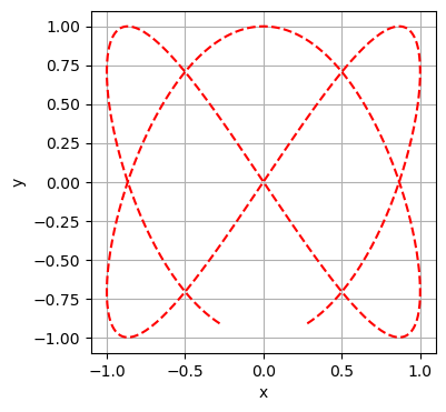

Lösung MF3: Gradient, Betrag des Gradienten

1. \(\nabla \phi=\begin{pmatrix} \partial \phi / \partial x \\ \partial \phi / \partial y \\ \partial \phi / \partial z \end{pmatrix} = \begin{pmatrix} 20 x y^3-5 y z^2 \\ 30 x^2 y^2-5 x z^2 \\ -10 x y z \end{pmatrix}\)

2. \(\left.\nabla \phi \right|_P=\begin{pmatrix} 0 \\ 10 \\ 20 \end{pmatrix} \rightarrow \left|\left.\nabla \phi \right|_P \right|=\sqrt{10^2+20^2}=\sqrt{500}=22.36\)

Lösung MF4: Divergenz eines Vektorfelds

1. div\(\mathbf{F}=\nabla \cdot \mathbf{F}=y^2+x^2-4=0 \rightarrow y^2+x^2=4 \rightarrow\) Die Divergenz verschwindet in jedem Punkt des Kreises mit Mittelpunkt im Ursprung und Radius 2.
2. Siehe Code

Code

x = np.arange(-5, 5, 1)
y = np.arange(-5, 5, 1)
X, Y = np.meshgrid(x,y)
U,V = [X*Y**2,X**2*Y-4*Y]

fig, ax = plt.subplots()
q = ax.quiver(X, Y, U, V)
circle=mpl.Circle((0,0),2,facecolor='none',ec='darkred')
ax.add_patch(circle)
ax.set_aspect('equal', adjustable='box')