Code
import numpy as np
import matplotlib.pyplot as plt
import sympy as sp
import numpy.linalg as linalgimport numpy as np
import matplotlib.pyplot as plt
import sympy as sp
import numpy.linalg as linalgplt.rcParams['figure.figsize']=(4,4)Sei \(v_1 = \begin{pmatrix}1 \\ 2 \\ 3 \end{pmatrix}, v_2 = \begin{pmatrix} 4 \\ 5 \\ 6 \end{pmatrix}\) und \(v_3 = \begin{pmatrix} 2 \\ 1 \\ 0 \end{pmatrix}\).
Betrachten Sie die lineare Funktion \(f:\mathbb{R}^2 \rightarrow \mathbb{R}: f(x) = 2x_1 - x_2\).
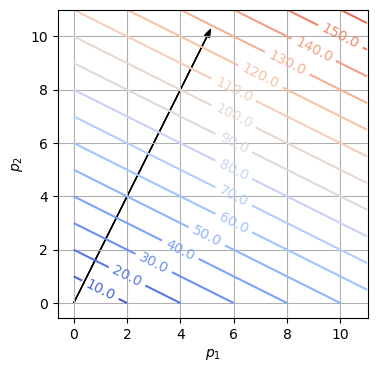
Wir nehmen an, daß die Temperatur \(T\) (gemessen über Raumtemperatur, beispielsweise \(T = 30\) Grad Celsius bedeutet 30 Grad Celsius über der Raumtemperatur) eines Computers mit zwei verschiedenen Prozessoren eine lineare Funktion der Leistungen \(p = (p_1, p_2)\) der zwei Prozessoren ist. Wenn beide Prozessoren im Leerlauf sind ist \(p = (2,2)\), was zu einer Temperatur \(T = 30\) Grad Celsius führt. Wenn der erste Prozessor mit voller Leistung arbeitet und die andere im Leerlauf ist, ist \(p = (8,2)\) und die Temperatur steigt auf \(T = 60\) Grad Celsius.
Die Vektoren \(v_i\) sind linear unabhängig, falls das lineare Gleichungssystem \(\alpha_1 v_1 + \alpha_2 v_2 + \alpha_3 v_3 = 0\) für die Koeffizienten \(\alpha_i \in \mathbb{R}\) nur die triviale Lösung \(\alpha_i = 0\) hat.
In komponenten ausgeschrieben lautet die Vektorgleichung \(\alpha_1 v_1 + \alpha_2 v_2 + \alpha_3 v_3 = 0\)
\[ \alpha_1 \begin{pmatrix} 1 \\ 2 \\ 3 \end{pmatrix} + \alpha_2 \begin{pmatrix} 4 \\ 5 \\ 6 \end{pmatrix} + \alpha_3 \begin{pmatrix} 2 \\ 1 \\ 0 \end{pmatrix} = \begin{pmatrix} 0 \\ 0 \\ 0 \end{pmatrix}. \]
In Gleichungsform:
\[\begin{align} \alpha_1 + 4 \alpha_2 + 2 \alpha_3 & = 0 \\ 2 \alpha_1 + 5 \alpha_2 + \alpha_3 & = 0 \\ 3 \alpha_1 + 6 \alpha_2 & = 0 \end{align}\]
In Matrixform:
\[\begin{pmatrix} 1 & 4 & 2 \\ 2 & 5 & 1 \\ 3 & 6 & 0 \end{pmatrix} \begin{pmatrix} \alpha_1 \\ \alpha_2 \\ \alpha_3 \end{pmatrix} = \begin{pmatrix} 0 \\ 0 \\ 0 \end{pmatrix}\]
Das lineare Gleichungssystem läßt sich z. B. mit dem Gaußschen Eliminationsverfahren lösen. Der Lösungsraum ist eindimensional und kann z. B. mit \(\alpha_3\) parametrisiert werden:
\[\begin{align} \alpha_1 & = 2 \alpha_3 \\ \alpha_2 & = - \alpha_3 \\ \alpha_3 & = \text{frei wählbar} \end{align}\]
Das lineare Gleichungssystem \(\alpha_1 v_1 + \alpha_2 v_2 + \alpha_3 v_3 = 0\) hat daher auch nicht-triviale Lösungen, z.B. mit \(\alpha_3 = -1\) gilt \(-2 v_1 + v_2 - v_3 = 0\). Daher sind die Vektoren linear abhängig.
# The command solve() can solve quadratic matrix equations Ax=b
# only when Ax=b has a unique solution. This is the case
# if and only if (short iff) the columns of A are linearly independent.
A = np.array([[1, 4, 2],
           [2, 5, 1],
           [3, 6, 0]])
b = np.zeros((3,1))
linalg.solve(A, b) # gives the trivial solution
array([[ 0.],
[ 0.],
[-0.]])# With the sympy package one can solve matrix equations Ax=b symbolically.
sp.init_printing() # initializes pretty-printing
a1, a2, a3 = sp.symbols('a1 a2 a3')
sp.linsolve([ a1 + 4*a2 + 2*a3,
2*a1 + 5*a2 + a3,
3*a1 + 6*a2 ],
(a1, a2, a3))\(\displaystyle \left\{\left( 2 a_{3}, \ - a_{3}, \ a_{3}\right)\right\}\)
# x1-x2-Grid:
delta = 0.25
x1 = np.arange(-5.0, 5.0, delta)
x2 = np.arange(-5.0, 5.0, delta)
X1, X2 = np.meshgrid(x1, x2)

# Koeffizientenvektor:
c = np.array([2, -1])
# c = array([2, -1])*3 # Skalieren von c damit die Konturlinien näher zueinander liegen
# c = array([2, -1])*0.2 # Skalieren von c damit die Konturlinien weiter voneinander liegen

# y = f(x) = c^T x:
Y = c[0]*X1 + c[1]*X2

# Plot:
plt.figure()
plt.axis('equal')
plt.arrow(0, 0, c[0], c[1], head_width=0.2, fc='k')
CS = plt.contour(X1, X2, Y, levels= [-2,0,2,4], cmap='coolwarm')
plt.clabel(CS, inline=1, fmt='%1.1f')
plt.xlabel('$x_1$')
plt.ylabel('$x_2$')
plt.grid(True)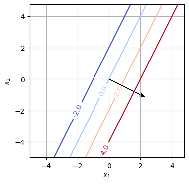
Die Temperatur wird als eine lineare Funktion der Leistungen \(p = (p_1, p_2)\) modelliert: \(T(p) = c_1 p_1 + c_1 p_2\). Einsetzen der zwei Messdaten in die Funktionsgleichung liefert:
\[\begin{align} c_1 2 + c_2 2 & = 30 \\ c_1 8 + c_2 2 & = 60 \end{align}\]
Das lineare Gleichungssystem ist eindeutig lösbar: \(c = \begin{pmatrix} 5 \\ 10 \end{pmatrix}\), siehe auch Code. Somit lautet die Funktionsgleichung \(T(p) = 5p_1 + 10p_2\).
Siehe Code.
Bei gleicher Leistung \(p\) beider Prozessoren gilt \(p_1 = p_2 =p\). Die Forderung, dass die Temperatur unter 90 Grad Celsius sei, bedeutet \(5p + 10p < 90\) und hat die Lösung \(p<6\). Somit kann die gleiche Leistung beider Prozessoren maximal 6 sein, damit die Temperatur unter 90 Grad Celsius ist.
# Solving the quadratic system of linear equations in matrix form with the command solve():
A = np.array([[2, 2],
           [8, 2]])
b = np.array([[30],
           [60]])
c = linalg.solve(A, b)
print(c)
[[ 5.]
[10.]]# contour lines of T(p) = 5p_1 + 10p_2:
delta = 1
p1 = np.arange(0, 12, delta)
p2 = np.arange(0, 12, delta)
P1, P2 = np.meshgrid(p1, p2)
T = c[0,0]*P1 + c[1,0]*P2
plt.figure()
plt.axis('equal')
plt.arrow(0, 0, c[0,0], c[1,0], head_width=0.2, fc='k')
CS = plt.contour(P1, P2, T, levels= np.arange(0, 200, 10), cmap= 'coolwarm') # colormaps()
plt.clabel(CS, inline=1, fmt='%1.1f')
plt.xlabel('$p_1$')
plt.ylabel('$p_2$')
plt.grid(True)