Code
import numpy as np
import matplotlib.pyplot as plt
import numpy.linalg as linalgimport numpy as np
import matplotlib.pyplot as plt
import numpy.linalg as linalgplt.rcParams['figure.figsize']=(4,4)Bestimmen Sie von Hand mit Hilfe des Gaußschen Eliminationsverfahrens, ob folgendes lineares Gleichungssystem nicht-triviale Lösungen hat.
\[\begin{align} 2x_1 - 5x_2 + 8x_3 & = 0 \\ -2x_1 - 7x_2 + x_3 & = 0 \\ 4x_1 + 2x_2 + 7x_3 & = 0 \end{align}\]
Überprüfen Sie Ihr Ergebnis am Computer mit Hilfe der Befehle det, inv, solve und matrix_rank.
Gegeben ist das lineare Gleichungssystem:
\[\begin{align} 2x_1 - 4x_2 - 2x_3 & = b_1 \\ -5x_1 + x_2 + x_3 & = b_2 \\ 7x_1 - 5x_2 - 3x_3 & = b_3 \end{align}\]
Hat das lineare Gleichungssystem für alle Vektoren \(b\) eine eindeutige Lösung? Wie können Sie dieses Problem am Computer lösen?
Chemische Reaktionsgleichungen beschreiben die Verhältnisse der Reaktanten und Produkte einer gegebenen Stoffumwandlung. Zum Beispiel reagiert bei der Verbrennung das Gas Propan (\(C_3 H_8\)) mit molekularem Sauerstoff (\(O_2\)) zu Kohlendioxid (\(CO_2\)) und Wasser (\(H_2 O\)), beschrieben durch die Reaktionsgleichung:
\[x_1 C_3 H_8 + x_2 O_2 \rightarrow x_3 CO_2 + x_4 H_2 O\]
Um die Reaktion ins Gleichgewicht zu bringen, gilt es die ganzzahligen Lösungen \(x_1,...,x_4\) zu finden, so dass die Gesamtzahlen von Kohlenstoff, Wasserstoff und Sauerstoff auf der rechten und linken Seite der Reaktionsgleichung übereinstimmen. Eine systematische Methode, um das Reaktionsgleichgewicht zu bestimmen, ist die Formulierung einer vektoriellen Gleichung, welche die Zahlen der Atome aller Elemente in der Reaktion beschreibt.
Überprüfen Sie, ob folgende vektorielle Gleichung die obige Reaktion beschreibt!
\[x_1 \begin{pmatrix} 3 \\ 8 \\ 0 \end{pmatrix} + x_2 \begin{pmatrix} 0 \\ 0 \\ 2 \end{pmatrix} = x_3 \begin{pmatrix} 1 \\ 0 \\ 2 \end{pmatrix} + x_4 \begin{pmatrix} 0 \\ 2 \\ 1 \end{pmatrix}.\]
Bestimmen Sie die Lösungsmenge in \(\mathbb{R}^4\).
Finden Sie die Lösung mit kleinstmöglichen ganzen Zahlen \(x_1,...,x_4\).
Der elektrische Schaltkreis in der folgenden Abbildung ist parametrisiert durch: \(U_1=230\), \(U_2=370\), \(R_1=200\), \(R_2=100\), \(R_3=300\).
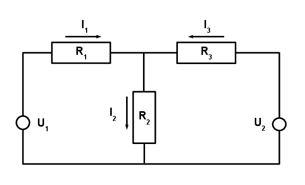 1. Formulieren Sie das lineare Gleichungssystem für die Stromstärken \(I_1\), \(I_2\), und \(I_3\) in Matrizenschreibweise \(Ax=b\). 2. Lösen Sie \(Ax=b\) händisch. 3. Lösen Sie \(Ax=b\) in Python mit dem Befehl
 solve. 4. Bestimmen Sie in Python die Determinante von \(A\) mit Hilfe des NumPy-Befehls det.
Überprüfen Sie, dass die Inverse einer 2x2 Matrix \(A = \begin{pmatrix} a & b\\ c & d \end{pmatrix}\) durch folgende Formel gegeben ist:
\[A^{-1} = \frac{1}{\det(A)}\begin{pmatrix} d & -b \\ -c & a \end{pmatrix} \text{ mit } \det(A) = ad - cb.\]
Benutzen Sie diese Formel, um die Inverse der Matrix \(A = \begin{pmatrix} 0.5 & 0\\ 0 & 3 \end{pmatrix}\) zu bestimmen. Beschreiben Sie die Abbildung \(f(x)=Ax\) in Worten.
Betrachten Sie die Rotationsmatrix
\[R = \begin{pmatrix} \cos(\alpha) & -\sin(\alpha) \\ \sin(\alpha) & \cos(\alpha) \end{pmatrix}.\]
Bestimmen Sie, ohne das linearen Gleichungssystem zu lösen, ob es lösbar ist und, falls ja, eindeutig lösbar ist.
\[\begin{pmatrix} -10 & 3 \\ -5 & 4 \end{pmatrix}\begin{pmatrix} x \\ y \end{pmatrix} = \begin{pmatrix} -3,5 \\ 9,2 \end{pmatrix}\]
Geben Sie ein Zahlenbeispiel für ein lineares Gleichungssystem in Matrixform an, das 2 Gleichungen, 3 Variablen und keine Lösung hat.
Geben Sie ein Zahlenbeispiel für ein lineares Gleichungssystem in Matrixform an, das mindestens 2 Gleichungen, mindestens 2 Variablen und einen 1-dimensionalen Lösungsraum hat.
Jedes Jahr ziehen etwa 10 % der Bevölkerung einer Stadt in die umliegenden Vororte, und etwa 20 % der Vorstadtbevölkerung in die Stadt. Im Jahr 2016 gibt es 10 Millionen Menschen in der Stadt und 8 Millionen Menschen in den Vororten, was wir mit dem Zustandsvektor \(x_0 = \begin{pmatrix} 10 \\ 8 \end{pmatrix}\) modellieren.
Quelle: David Lay, Linear Algebra and Its Applications, 4th edition, p.87, exercise 10
Sind die folgenden drei Vektoren linear abhängig oder linear unabhängig? Begründen Sie Ihre Antwort.
\[\begin{pmatrix} 2 \\ 1 \\ 0 \end{pmatrix}, \begin{pmatrix} -1 \\ 2 \\ 5 \end{pmatrix}, \begin{pmatrix} -1 \\ 2 \\ -1 \end{pmatrix}\]
Zeigen Sie, dass die Matrix \(A = \begin{pmatrix} \frac{1}{\sqrt{2}} & \frac{1}{\sqrt{2}} \\ -\frac{1}{\sqrt{2}} & \frac{1}{\sqrt{2}} \end{pmatrix}\) orthogonal ist, d. h. dass \(A^T=A^{-1}\) gilt.
Gegeben ist die Matrix \(A= \left( \begin{matrix} 1&0&2 \\ 0&2&0 \\ 0&1&3 \end{matrix} \right)\).
Hinweis:
\[\det \begin{pmatrix} a_{11} & a_{12} & a_{13} \\ a_{21} & a_{22} & a_{23} \\ a_{31} & a_{32} & a_{33} \end{pmatrix} = a_{11} a_{22} a_{33} +a_{12} a_{23} a_{31} + a_{13} a_{21} a_{32} - a_{13} a_{22} a_{31} - a_{12} a_{21} a_{33} - a_{11} a_{23} a_{32},\]
Bestimmen Sie, ohne das Gleichungssystem zu lösen, ob eine Lösung existiert.
\[\begin{pmatrix} -10 & 3 \\ -5 & 4 \end{pmatrix}\begin{pmatrix} x_1 \\ x_2 \end{pmatrix} = \begin{pmatrix} -3.5 \\ 9.2 \end{pmatrix}\]
Für welche Werte von \(h\) sind die folgenden Vektoren linear abhängig?
\[\begin{pmatrix} 1 \\ -2 \\ -4 \end{pmatrix}, \begin{pmatrix} -3 \\ 7 \\ 6 \end{pmatrix}, \begin{pmatrix} 2 \\ 1 \\ h \end{pmatrix}\]
Hinweis:
\[\det \begin{pmatrix} a_{11} & a_{12} & a_{13} \\ a_{21} & a_{22} & a_{23} \\ a_{31} & a_{32} & a_{33} \end{pmatrix} = a_{11} a_{22} a_{33} +a_{12} a_{23} a_{31} + a_{13} a_{21} a_{32} - a_{13} a_{22} a_{31} - a_{12} a_{21} a_{33} - a_{11} a_{23} a_{32},\]
Bestimmen Sie von Hand und in Python alle Eigenwerte und -vektoren folgender Matrix.
\[\begin{pmatrix} 2 & 7 \\ 7 & 2 \end{pmatrix}\]
Bestimmen Sie alle Eigenwerte und -vektoren folgender Matrix.
\[\begin{pmatrix} -2 & -5 \\ 1 & 4 \end{pmatrix}\]
Quelle: Papula, Band 2, 7.2, S. 128 f.
Das Gaußschen Eliminationsverfahrens liefert, dass das Gleichungssystem nicht-triviale Lösungen hat, nämlich alle Vielfachen von \(x = \begin{pmatrix} -17 \\ 6 \\ 8 \end{pmatrix}.\) Siehe auch Code.
# matrix form Ax=b of the system of linear equations:
A = np.array([[ 2, -5, 8],
           [-2, -7, 1],
           [ 4,  2, 7]])
b = np.zeros((3,1))

# check if (-17, 6, 8) is a solution:
x = np.array([-17, 6, 8])
print("Ax = {}".format(A@x)) # should be zero as the system is Ax=0

# From det(A) = 0 it follows that Ax=0 has infinitly many solutions:
print("Determinante = {}".format(linalg.det(A)))

# Erinnerung: Rang einer Matrix = Anzahl der linear unabhängigen Spalten- oder Zeilenvektoren
# Ax=b  hat unendlich viele Lösungen, wenn Rang(A)=Rang(A|b)<Anzahl Variablen.
print("Rang(A)  =", linalg.matrix_rank(A))
Ab = np.hstack((A, b))
print("Rang(Ab) =", linalg.matrix_rank(Ab))
# Conlusion: Ax=b has infinitly many solutions.

# linalg.inv(A)         # -> LinAlgError: Singular matrix, can also be seen from det(A)=0

# linalg.solve(A, b)    # -> LinAlgError: Singular matrix, can also be seen from det(A)=0
Ax = [0 0 0]
Determinante = 0.0
Rang(A) = 2
Rang(Ab) = 2Siehe Code. Das lineare Gleichungssystem \(Ax=b\) hat nicht für alle Vektoren \(b\) eine eindeutige Lösung, denn der Rang von \(A\) ist kleiner als die Anzahl an Spalten von \(A\), bzw. die Determinante von \(A\) ist Null.
A = np.array([[ 2, -4, -2],
           [-5,  1,  1],
           [ 7, -5, -3]])
print("rank(A) = {}".format(linalg.matrix_rank(A)))
print("det(A)  = {}".format(linalg.det(A)))
rank(A) = 2
det(A) = 5.709718412357936e-16Die vektorielle Gleichung entspricht den Massenbilanzen für die drei Elemente \(C\), \(H\) und \(O\).
Das Gaußschen Eliminationsverfahren liefert, dass das lineare Gleichungssystem eine 1-dimensionale Lösungsmenge hat, die z. B. mit \(x_4\) parametrisiert werden kann:
\[\begin{align} x_4 & = \text{frei wählbar} \\ x_3 & = 0.75 x_4 \\ x_2 & = 1.25 x_4 \\ x_1 & = 0.25 x_4 \end{align}\]
Lösung mit kleinstmöglichen ganzen Zahlen: \(x_1 = 1, x_2 = 5, x_3 = 3,x_4 = 4\).
Das lineare Gleichungssystem
\[\begin{align} I_1 - I_2 + I_3 & = 0 \\ R_1 I_1 + R_2 I_2 & = 230 \\ R_2 I_2 + R_3 I_3 & = 370 \end{align}\]
hat die eindeutige Lösung \(I_1=0.5\), \(I_1=1.3\), \(I_3=0.8\), siehe auch Code.
Die Matrixform lautet
\[\begin{pmatrix} 1 & -1 & 1 \\ R_1 & R_2 & 0 \\ 0 & R_2 & R_3 \end{pmatrix} \begin{pmatrix} I_1 \\ I_2 \\ I_3 \end{pmatrix} = \begin{pmatrix} 0 \\ 230 \\ 370 \end{pmatrix}\]
# matrix form:
A = np.array([[  1,  -1,   1],
           [200, 100,   0],
           [  0, 100, 300]])
b = np.array([0, 230, 370])

# det(A) is not zero. Therefore, Ax=b has a unique solution.
print("det(A) = {}".format(linalg.det(A)))

# The unique solution can be computed via solve():
I = linalg.solve(A, b)
print("I = {}".format(I))
det(A) = 109999.99999999991
I = [0.5 1.3 0.8]A = np.array([[0.5, 0],
[0 , 3]])
print("inv(A) = \n{}".format(linalg.inv(A)))inv(A) =
[[2. 0. ]
[0. 0.33333333]]alpha = np.pi/6
R = np.array([[np.cos(alpha), -np.sin(alpha)],
[np.sin(alpha), np.cos(alpha)]])
print("R = \n{}".format(R))
print("R^T R = \n{}".format(R.T@R))
print("det(R) = {}".format(linalg.det(R)))
print("inv(R) = \n{}".format(linalg.inv(R)))R =
[[ 0.8660254 -0.5 ]
[ 0.5 0.8660254]]
R^T R =
[[1.00000000e+00 7.43708407e-18]
[7.43708407e-18 1.00000000e+00]]
det(R) = 1.0
inv(R) =
[[ 0.8660254 0.5 ]
[-0.5 0.8660254]]A = np.array([[-10, 3],
[ -5, 4]])
print("det(A) = {}".format(linalg.det(A))) # is negative => Ax=b has a unique solution.det(A) = -25.000000000000007# initial state_
x0 = np.array([[10],
[8]])
# transition matrix:
M = np.array([[0.9, 0.2],
[0.1, 0.8]])
# dynamics:
n = 50 # number of years
times = np.arange(n) # vector of years from now
X = np.zeros((2,n)) # matrix with states as columns
X[:,[0]] = x0 # put initial state into first column
for k in range(1, n): # iterate over years
X[:,[k]] = M@X[:,[k - 1]]plt.figure(figsize=(5,3))
plt.plot(times, X[0,:], '.-', label='Stadt')
plt.plot(times, X[1,:], '.-', label='Vororte')
plt.legend(loc='best')
plt.xlabel('Zeit [Jahr]')
plt.ylabel('Anzahl Menschen [Mio.]')
plt.ylim(0,13)
plt.grid(True)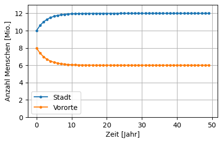
# eigenvalues and eigenvectors:
L, V = linalg.eig(M)
print("eigenvalues = {}".format(L))
print("matrix with eigenvectors in columns = \n{}".format(V))
eigenvalues = [1. 0.7]
matrix with eigenvectors in columns =
[[ 0.89442719 -0.70710678]
[ 0.4472136 0.70710678]]# rescaling of eigenvestors:
e0 = V[:,[0]] # first column
e0 = e0/np.sum(e0)
e1 = np.array([[-1],
[ 1]])
E = np.hstack((e0, e1))
print("matrix with rescaled eigenvectors in columns = \n{}".format(E))matrix with rescaled eigenvectors in columns =
[[ 0.66666667 -1. ]
[ 0.33333333 1. ]]# representation of the initial state x0 as a linear combination of the eigenvectors:
# y00*e0 + y10*e1 = E*y0 = x0, with y0 the column vector of the coefficients
y0 = linalg.solve(E, x0)
print("y0 = \n{}".format(y0))y0 =
[[18.]
[ 2.]]# The part of the linear combination belonging to eigenvalue 1 dominates.
# and forms the limit value for large times, see figure above.:
print(y0[0,0]*e0)[[12.]
[ 6.]]Lineare Unabhängigkeit der Vektoren \(v_i\) ist gegeben, wenn das lineare Gleichungssystem \(x_1 v_1 + x_2 v_2 + x_3 v_3 = 0\) nur die triviale Lösung \(x=0\) hat. Lösen des zugehörigen Gleichungssystems in Matrixform \(Ax=0\) (von Hand oder mit dem Computer) zeigt, dass es nur die triviale Lösung \(x=0\) hat. Alternativ kann mit der Determinante oder dem Rang argumentiert werden, siehe Code.
A = np.array([[2,-1,-1],
           [1, 2, 2],
           [0, 5,-1]])

print("det(A) = {}".format(linalg.det(A)))
# not zero => there is a unique solution to Ax=0, namely the trivial x=0

print("rank(A) = {}".format(linalg.matrix_rank(A)))
# rank(A) = rang(A|b) = n =>
# there is a unique solution to Ax=0, namely the trivial x=0
det(A) = -29.99999999999999
rank(A) = 3Händisches Nachrechnen ergibt \(A^T A = I\) und \(AA^T = I\), was die Behauptung beweist. Siehe auch Code.
A = np.array([[ 1/np.sqrt(2), 1/np.sqrt(2)],
           [-1/np.sqrt(2), 1/np.sqrt(2)]])

print(A.T - linalg.inv(A))  # should be the zero matrix
# Note that the typical numerical precision on a computer is at the level 1e-16.
[[-1.11022302e-16 1.11022302e-16]
[-1.11022302e-16 -1.11022302e-16]]A = np.array([[1, 0, 2],
[0, 2, 0],
[0, 1, 3]])
L, V = linalg.eig(A)
print("eigenvalues of A: {}".format(L))
print("matrix with eigenvectors of A in columns: \n{}".format(V))
print("det(A) = {}".format(linalg.det(A)))eigenvalues of A: [1. 3. 2.]
matrix with eigenvectors of A in columns:
[[ 1. 0.70710678 -0.81649658]
[ 0. 0. 0.40824829]
[ 0. 0.70710678 -0.40824829]]
det(A) = 6.0Ja, denn die Determinante der Koeffizientenmatrix ist nicht Null.
A = np.array([[-10, 3],
           [ -5, 5]])
print("det(A) = {}".format(linalg.det(A)))
det(A) = -35.00000000000001Die Determinante der Vektoren-Matrix berechnet sich zu \(h+38\). Die Determinante ist für nur für \(h=-38\) Null. Für diesen Wert von \(h\) sind die Vektoren linear abhänging.
h = -38
A = np.array([[ 1, -3, 2],
           [-2,  7, 1],
           [-4,  6, h]])
print("det(A) = {}".format(linalg.det(A)))
det(A) = 0.0Die zwei Lösungen \(\lambda_i\) von \(\det(A - \lambda I)\) sind die Eigenwerte von \(A\): \(\lambda_1 = -5, \lambda_2 = 9\). Die zwei dazugehörigen Eigenvektoren \(v_i\) sind die Lösungen der linearen Gleichungssysteme \(A v_i = \lambda v_i\): z. B. \(v_1 = (-1,1)^T, v_2 = (1,1)^T\). Siehe auch Code.
A = np.array([[2, 7],
           [7, 2]])
L, V = linalg.eig(A)

print("eigenvalues of A: {}".format(L))
print("matrix with eigenvectors of A in columns: \n{}".format(V))
eigenvalues of A: [ 9. -5.]
matrix with eigenvectors of A in columns:
[[ 0.70710678 -0.70710678]
[ 0.70710678 0.70710678]]Die zwei Lösungen \(\lambda_i\) von \(\det(A - \lambda I)\) sind die Eigenwerte von \(A\): \(\lambda_1 = -1\), \(\lambda_2 = 3\), Die zwei dazugehörigen Eigenvektoren \(v_i\) sind die Lösungen der linearen Gleichungssysteme \(A v_i = \lambda v_i\): \(v_1 = (-5, 1)^T\), \(v_2 = (-1, 1)^T\) Siehe auch Code.
A = np.array([[-2, -5],
           [ 1,  4]])
L, V = linalg.eig(A)

print("eigenvalues of A: {}".format(L))

print("rescaled 1st eigenvector: \n{}".format(V[:,[0]]/np.sum(V[1,0])))
print("rescaled 2nd eigenvector: \n{}".format(V[:,[1]]/np.sum(V[1,1])))
eigenvalues of A: [-1. 3.]
rescaled 1st eigenvector:
[[-5.]
[ 1.]]
rescaled 2nd eigenvector:
[[-1.]
[ 1.]]