Code
import numpy as np
import matplotlib.pyplot as plt
import numpy.linalg as linalg
from scipy.optimize import linprogimport numpy as np
import matplotlib.pyplot as plt
import numpy.linalg as linalg
from scipy.optimize import linprogLaden Sie mit folgenden Python-Befehlen die Daten der Datei Polyfit.csv in ein array D, dessen Spalten als Daten-Vektoren \(t\) und \(y\) weiterverwendet werden:
D = genfromtxt('Polyfit.csv', delimiter=';')
t = D[:,0]
y = D[:,1]lstsq), um ein Polynom vom Grad 4 durch die Punktwolke zu fitten. Erzeugen Sie ein Stamm-Blatt-Diagramm der Koeffizienten. Warum sind die ungeraden Koeffizienten null?polyfit und poly1d um die gleichen Resultate zu erzielen.Mehr Information zum Beispiel unter https://de.wikipedia.org/wiki/Mooresches_Gesetz.
D = genfromtxt('Moores_Law.csv', delimiter=';')
t = D[:,0]
n = D[:,1]
und plotten Sie \(n\) gegen \(t\) mit den Befehlen plot und semilogy. 2. Erklären Sie, wie die Methode der kleinsten Fehlerquadrate (Reggression) verwendet werden kann, um \(\alpha\) und \(t_0\) zu bestimmen, so dass
\[n_i \approx \alpha^{t_i -t_0} \text{ for } i= 1, . . . , 13\]
gilt. 3. Lösen Sie das Least-Squares-Problem (d.h. die Reggressionsaufgabe) in Python mit dem Befehl lstsq. Vergleichen Sie Ihre Resultate mit dem Mooreschen Gesetz, das behauptet, dass sich die Anzahl der Transistoren in Mikroprozessoren alle 2 Jahre verdoppelt.
Die Müllmenge in Millionen Tonnen pro Tag des Landes Lower Slobbovia von 1960 bis 1995 ist in folgender Tabelle wiedergegeben.
| Jahr \(t\) | 1960 | 1965 | 1970 | 1975 | 1980 | 1985 | 1990 | 1995 |
|---|---|---|---|---|---|---|---|---|
| Menge \(y\) | 86.0 | 99.8 | 135.8 | 155.0 | 192.6 | 243.1 | 316.3 | 469.5 |
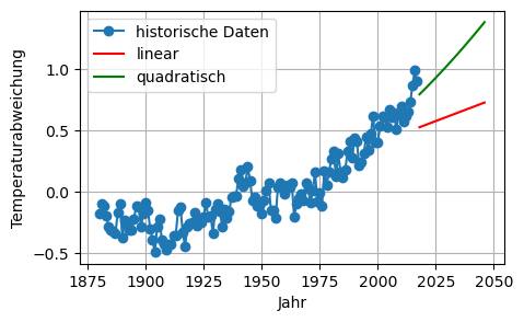
Laden Sie die Datei Global_Temperatures.csv in Python mit dem Befehl:
D = genfromtxt('Global_Temperatures.csv', delimiter=';')Die Werte stammen von der NASA-Homepage GISS Surface Temperature Analysis. Sie repräsentieren jährliche Mittel der Abweichungen der Oberflächentemperaturen vom Mittel der Jahre 1951 bis 1980. Die erste Spalte enthält die Jahre, die zweite die jährlichen Mittelwerte, die dritte die 5-jährlichen Mittelwerte.
Laden der Daten, Berechnung und Darstellung der Regressionskoeffizienten:
D = np.genfromtxt('daten/Polyfit.csv', delimiter=';')
t = D[:,0]
y = D[:,1]
n = len(t)

A = np.column_stack( (np.ones((n, 1)), t, t**2, t**3, t**4) )
x = linalg.lstsq(A, y, rcond=None)[0]

for k in range(len(x)):
    print("Koeffizient der Ordnung {:d} = {:10.6f}".format(k, x[k]))

plt.figure(figsize=(5,3))
plt.stem(x)
plt.xlabel('x')
plt.xlim(-1, 5)
plt.grid(True)
Koeffizient der Ordnung 0 = 0.661640
Koeffizient der Ordnung 1 = -0.000000
Koeffizient der Ordnung 2 = -0.087919
Koeffizient der Ordnung 3 = 0.000000
Koeffizient der Ordnung 4 = 0.002735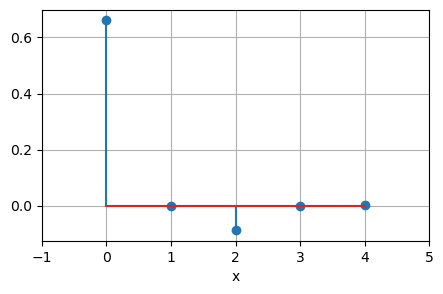
Plot des polynomialen Fits:
y_fit = A@x

plt.figure(figsize=(5,3))
plt.plot(t, y, 'o', label='Datenpunkte')
plt.plot(t, y_fit, '-r', label='Fit')
plt.xlabel('t')
plt.ylabel('y')
plt.legend(numpoints = 1)
plt.grid(True)
Befehle polyfit und poly1d:
ordnung = 4
c = np.polyfit(t, y, ordnung)

for k in range(ordnung + 1):
    print("Koeffizient der Ordnung {:d} = {:10.6f}".format(ordnung - k, c[k]))

plt.figure(figsize=(5,3))
plt.plot(t, y, 'o',label='Datenpunkte')
plt.plot(t, np.poly1d(c)(t),'-r',label='Fit')
plt.xlabel('t')
plt.ylabel('y')
plt.legend()
plt.grid(True)
Koeffizient der Ordnung 4 = 0.002735
Koeffizient der Ordnung 3 = 0.000000
Koeffizient der Ordnung 2 = -0.087919
Koeffizient der Ordnung 1 = -0.000000
Koeffizient der Ordnung 0 = 0.661640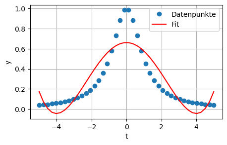
D = np.genfromtxt('daten/Moores_Law.csv', delimiter=';')
t = D[:,0]
n = D[:,1]plt.figure(figsize=(6,6))
plt.subplot(211)
plt.plot(t, n, 'o-')
plt.xlabel("t (Jahr)")
plt.ylabel("n (Anzahl Transistoren)")
plt.grid(True)
plt.subplot(212)
plt.semilogy(t,n,'o-')
plt.xlabel("t (Jahre)")
plt.ylabel("n (Anzahl Transistoren)")
plt.grid(True)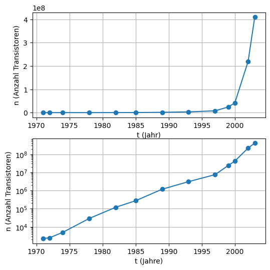
\[\begin{align} n_i & = \alpha^{(t_i - t_0)} | \log() \\ \log(n_i) & = (t_i - t_0)\log(\alpha) \\ \log(n_i) & = -t_0\log(\alpha) + \log(\alpha)t_i \end{align}\]
b = np.log(n)
m = len(b)
A = np.column_stack((np.ones((m, 1)), t))
x = linalg.lstsq(A, b, rcond=None)[0]

alpha = np.exp(x[1])
t0 = -x[0]/x[1]
n_fit= alpha**(t - t0)

print("t0 = ", t0)
print("alpha^2 = ", alpha**2)
t0 = 1949.7063396217347
alpha^2 = 2.0325271695788167plt.figure(figsize=(5,3))
plt.semilogy(t, n, 'o')
plt.semilogy(t, n_fit, '-');
plt.xlabel("t (Jahr)")
plt.ylabel("n (Anzahl Transistoren)")
plt.grid(True)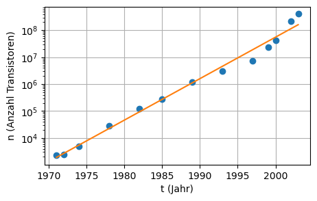
Minimiere \(\sum_{t=1960}^{1995} (y_t - (kt + d))^2\) in Matrixform:
\[\text{min. }\lVert\begin{pmatrix} 1960 & 1 \\ 1965 & 1 \\ \vdots & \vdots \\ 1995 & 1 \end{pmatrix} \begin{pmatrix} k \\ d \end{pmatrix} - \begin{pmatrix} 86.0 \\ 99.8 \\ \vdots \\ 469.5 \end{pmatrix} \rVert\]
Logarithmieren von \(y=ce^{\alpha t}\) liefert \(\ln(y) = \alpha t + \ln(c)\).
\[\text{min. }\lVert\begin{pmatrix} 1960 & 1 \\ 1965 & 1 \\ \vdots & \vdots \\ 1995 & 1 \end{pmatrix} \begin{pmatrix} \alpha \\ \ln(c) \end{pmatrix} - \begin{pmatrix} \ln(86.0) \\ \ln(99.8) \\ \vdots \\ \ln(469.5) \end{pmatrix} \rVert\]
Siehe Code -> exponentielles Modell
t = np.arange(1960, 2000, 5)
y = np.array([86.0, 99.8, 135.8, 155.0, 192.6, 243.1, 316.3, 469.5])

plt.figure(figsize=(5,3))
plt.plot(t, y, 'o-')
plt.xlim(1955, 2000)
plt.xlabel('Jahr')
plt.ylabel('Menge [Mio. t pro Tag]')
plt.grid(True)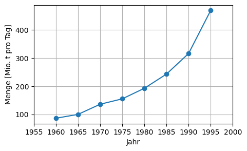
# linear, d. h. Gerade:
n = len(t)
A = np.column_stack( (np.ones((n,1)),t) )
x_linear = linalg.lstsq(A, y, rcond=None)[0]
y_fit_linear = np.dot(A, x_linear)

# exponentiell:
A = np.column_stack( (np.ones((n,1)),t) )
x_exp = linalg.lstsq(A, np.log(y), rcond=None)[0]
y_fit_exp = np.exp(np.dot(A, x_exp))

plt.figure(figsize=(5, 3))
plt.plot(t, y, 'o-', label='historische Daten')
plt.plot(t, y_fit_linear, '.-r', label='linearer Fit')
plt.plot(t, y_fit_exp   , '.-g', label='exponentieller Fit')
plt.xlabel('Jahr')
plt.ylabel('Temperaturabweichung')
plt.legend(loc='best', numpoints=1)
plt.grid(True)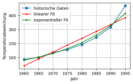
D = np.genfromtxt('daten/Global_Temperatures.csv', delimiter=';')
t = D[:,0]
T = D[:,1]
n = len(t)plt.figure(figsize=(5,3))
plt.plot(t, T, 'o-', label='historische Daten')
plt.xlabel('Jahr')
plt.ylabel('Temperaturabweichung')
plt.legend(numpoints=1, loc='best')
plt.grid(True)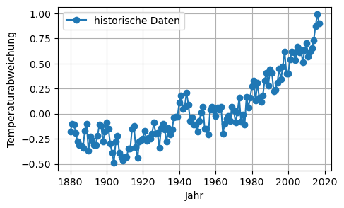
Linearer (Gerade) und quadratischer Fit via Least-Squares:
# linear, d. h. Gerade:

A = np.column_stack( (np.ones((n,1)),t) )
x_linear = linalg.lstsq(A, T, rcond=None)[0]
y_fit_linear = A@x_linear

# quadratisch:
A = np.column_stack( (np.ones((n,1)),t,t**2) )
x_quadr = linalg.lstsq(A, T, rcond=None)[0]
y_fit_quadr = A@x_quadr

plt.figure(figsize=(5,3))
plt.plot(t, T, 'o-', label='historische Daten')
plt.plot(t, y_fit_linear, '-r', label='linearer Fit')
plt.plot(t, y_fit_quadr , '-g', label='quadratischer Fit')
plt.xlabel('Jahr')
plt.ylabel('Temperaturabweichung')
plt.legend(loc='best', numpoints=1)
plt.grid(True)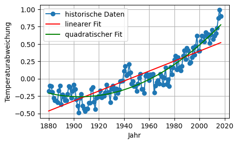
Prognosen:
t_ = np.arange(2018, 2047)
n_ = len(t_)

# linear:
A_ = np.column_stack( (np.ones((n_,1)),t_) )
y_prog_linear = A_ @ x_linear

# quadratisch:
A_ = np.column_stack( (np.ones((n_,1)),t_,t_**2) )
y_prog_quadr = A_ @ x_quadr

plt.figure(figsize=(5,3))
plt.plot(t, T, 'o-', label='historische Daten')
plt.plot(t_, y_prog_linear, '-r', label='linear')
plt.plot(t_, y_prog_quadr , '-g', label='quadratisch')
plt.xlabel('Jahr')
plt.ylabel('Temperaturabweichung')
plt.legend(numpoints=1, loc = 'best')
plt.grid(True)