Code
import numpy as np
import matplotlib.pyplot as plt
from scipy.integrate import odeint
import sympy as spimport numpy as np
import matplotlib.pyplot as plt
from scipy.integrate import odeint
import sympy as spplt.rcParams['figure.figsize']=(5,3)Zeigen Sie, dass die Funktion \(y(x) = C\frac{x}{1 + x}\) die allgemeine Lösung der Differentialgleichung \(x(1+x)y'(x) - y(x) = 0\) ist. Wie lautet die partikuläre Lösung zum Anfangswert \(y(1)=8\)? Erstellen Sie in Python einen Plot der partikulären Lösung.
Die Aufladung eines Kondensators der Kapazität \(C\) ab dem Zeitpunkt \(t=0\) über einen ohmschen Widerstand \(R\) auf die Endspannung \(u_0\) erfolgt nach dem Exponentialgesetz \(u_C(t) = u_0 (1- e^{-\frac{t}{RC}})\). Skizzieren Sie die Funktion \(u_C(t)\). Zeigen Sie, dass diese Funktion eine partikuläre Lösung der Differentialgleichung \(RC\dot{u_C}(t) + u_C(t) = u_0\) ist, die diesen Einschaltvorgang beschreibt. Erstellen Sie in Python Plots der Funktion \(u_C(t)\) für verschiedene Werte von \(C\) und \(R\).
Quellen:
Lösen Sie folgende DGL mit der Methode der Trennung der Variablen und überprüfen Sie jeweils Ihre Ergebnisse am Computer mittels SymPy.
Quellen:
Überprüfen Sie, ob die DGL exakt ist, und lösen Sie das Anfangswertproblem.
\[\dot{y} = \frac{-y^2}{2yt + 1}, \quad y(1)=-2\]
Quelle: Bronson: Schaum’s “Differential Equations”, p.36
Gegeben ist die Differentialgleichung \(y' = \frac{-2xy}{1 + x^2}\).
Quelle: Bronson: Schaum’s “Differential Equations”, Aufgaben 5.2 und 5.11, S. 33 und 36
Lösen Sie das folgende Anfangswertproblem \(yy' = \cos(2x), y(0) = -1\).
Ist die Differentialgleichung \(\dot{y}(t) = \frac{t + \sin(y(t))}{2y(t) - t\cos(y(t))}\) exakt? Begründen Sie Ihre Antwort. Geben Sie die allgemeine Lösung der Differentialgleichung in impliziter Form an.
Ein Auto mit Masse \(m\) und Anfangsgeschwindigkeit \(v_0\) bewegt sich nur unter dem Einfluss des als quadratisch von der Geschwindigkeit abhängig angenommenen Luftwiderstands.
Lösen Sie das Anfangswertproblem
\[y' = \frac{-x}{y}, \; y(0)=1.\]
Quelle: Farlow: Introduction to Differential Equations. Example 3, p. 40f.
x = np.linspace(1, 10)
y = 16*x/(1 + x)

plt.figure()
plt.plot(x, y,'r')
plt.xlabel('x')
plt.ylabel('y')
plt.grid(True)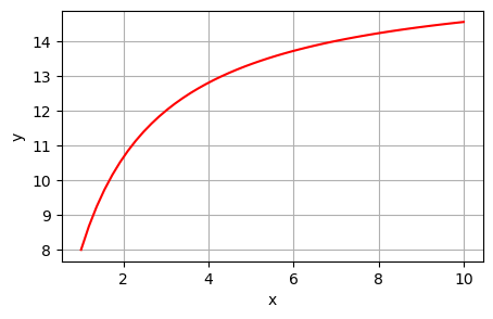
t = np.linspace(0, 10)
R = 1
C = 1
u0 = 1
u = u0*(1 - np.exp(-t/(R*C)))

plt.figure()
plt.plot(t, u,'r')
plt.xlabel('t')
plt.ylabel('u')
plt.grid(True)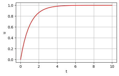
t = sp.symbols('t')
y = sp.symbols('y', cls=sp.Function)sp.init_printing()
diffeq = sp.Eq(y(t)*y(t).diff(t), t*sp.exp(t))
diffeq\(\displaystyle y{\left(t \right)} \frac{d}{d t} y{\left(t \right)} = t e^{t}\)
sp.dsolve(diffeq, y(t))\(\displaystyle \left[ y{\left(t \right)} = - \sqrt{2} \sqrt{C_{1} + t e^{t} - e^{t}}, \ y{\left(t \right)} = \sqrt{2} \sqrt{C_{1} + t e^{t} - e^{t}}\right]\)
diffeq = sp.Eq(y(t).diff(t)*(1 + t**2), t*y(t))
diffeq
\(\displaystyle \left(t^{2} + 1\right) \frac{d}{d t} y{\left(t \right)} = t y{\left(t \right)}\)
sp.dsolve(diffeq, y(t))\(\displaystyle y{\left(t \right)} = C_{1} \sqrt{t^{2} + 1}\)
sp.init_printing(False)sp.init_printing(use_unicode=True)
diffeq = sp.Eq(y(t).diff(t), -y(t)**2/(2*y(t)*t + 1))
diffeq\(\displaystyle \frac{d}{d t} y{\left(t \right)} = - \frac{y^{2}{\left(t \right)}}{2 t y{\left(t \right)} + 1}\)
sp.dsolve(diffeq, y(t))\(\displaystyle \left[ y{\left(t \right)} = \frac{- \sqrt{C_{1} t + 1} - 1}{2 t}, \ y{\left(t \right)} = \frac{\sqrt{C_{1} t + 1} - 1}{2 t}\right]\)
sp.init_printing(False)\(y(x) = -\sqrt{\sin(2x) + 1}\)
\(\frac{t^2}{2} + t\sin(y) - y^2 = c\)
t = np.linspace(0, 60*5) # seconds
v0 = 30               # meters per second
m = 1000              # kg
c = 1.0

v = v0/(1 + c*v0/m*t)

plt.figure()
plt.plot(t, v,'r')
plt.xlabel('t')
plt.ylabel('v')
plt.grid(True)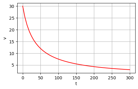
ist exakt, \(y=\sqrt{1 - x^2}\)