import numpy as np
import pandas as pd
import matplotlib.pyplot as plt
from importlib import reload

import solar
reload(solar)


sdo = pd.read_csv('solar_Dornbirn.csv', parse_dates=True, index_col='datetime')
print(sdo)Assignment #08
Unit 08
Until next week, work through the material provided in Unit 8 and solve the following exercise.
This week focuses on solving complex, real-world tasks using gridded data and visualizing your results. This exercise provides yet another opportunity to enhance your proficiency in matrix indexing and for-loops.
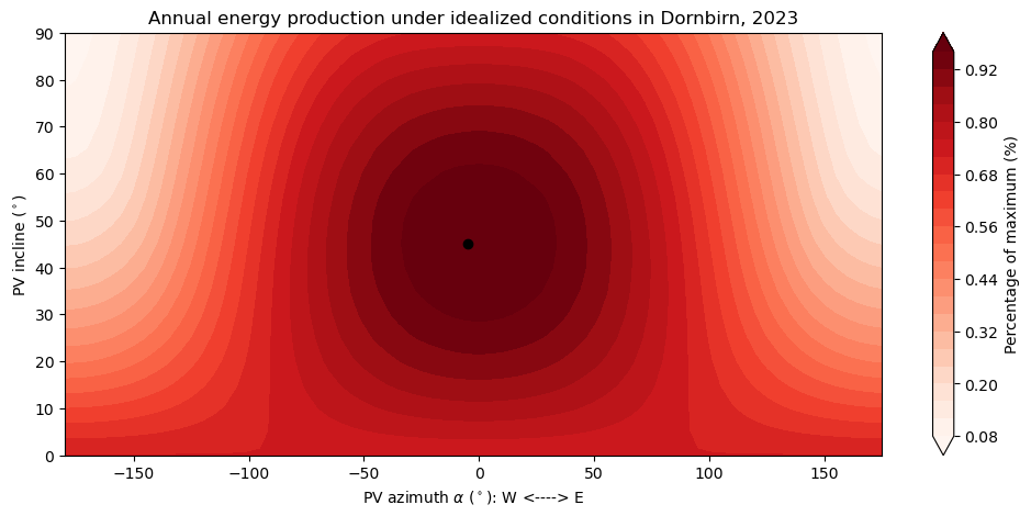
Exercise #08-01: Grid search
A grid search involves systematically searching through a predefined set of parameters to find the best parameter configuration for a specific question or model.
We aim to determine how the azimuth angle and incline of a PV module impact its energy production. We can utilize our existing solar module to address this question under idealized conditions and simplified assumptions.
Try to reproduce the following figure as closely as possible. Below, you will find some starting points for your code.
Before you get started with your own code, make sure you download my version of the solar module that implements the set of equations from last unit and the spreadsheet solar_Dornbirn.csv that contains information about the position of the sun and its irradiance over one year in Dornbirn.
After you have done that, start a notebook and try to solve the task. The following code blocks give you some starting points.
We will perform the grid search by calling a function that implements the required computations at each iteration for us. In other words, this function computes the energy produced by the PV module. In the following, I define that function and within the function body I have left you an opportunity for exercise. This task is not essential to continue with the remaining tasks. Do not get hung up here. Tip: Use the method pd.Series.diff() and the timedelta method .dt.total_seconds() to compute the time sampling in hours. If the time sampling is not equal between all time steps, raise an error.
You can either put the function into solar or directly into your notebook.
Energy generated by a PV module. The function implements the following physical considerations:
The power \(P\) generated by a PV module is the irradiance G (W/m2) multiplied by the area of the module A (m2) and the efficiency of the module \(\eta\), which in turn depends on temperature and a variety of other things. Let’s simplify and use \(\eta = 0.2\) for this exercise. The energy E generated by the module is then \(E = \sum P \cdot \Delta t\), where \(\Delta t\) is the sampling interval.
## Define a function that will compute the energy produced by the PV module
def comp_energy_produced(iswr0, beta, pvazimuth, elevangle, azimuth, datetime = None, efficiency=0.2, area=1):
    """
    Calculate the energy produced by a PV module based on solar irradiance data.

    Parameters
    ----------
    iswr0 (pandas.Series): Solar irradiance data onto horizontal surface.
    beta (float): Incline angle of the PV module (in degrees).
    pvazimuth (float): Azimuth angle of the PV module (in degrees, 0 in the south).
    elevangle (array-like): Elevation angle of the sun (in degrees).
    azimuth (array-like): Azimuth angle of the sun (in degrees, 0 in the south).
    datetime (pandas.Series or None, optional): Timestamps associated with the irradiance data. If None,
        the function assumes regular time intervals based on the index of 'iswr0'.
    efficiency (float, optional): Efficiency of the photovoltaic system (default is 0.2).
    area (float, optional): Area of the PV module (default is 1).

    Returns
    -------
    float: Total energy produced by the photovoltaic system (in Wh).

    If 'datetime' is not provided, the function assumes regular time intervals based on the index of 'iswr0'.
    The function raises a ValueError if the time intervals are irregular.
    """

    if datetime is None:
        datetime = iswr0.index.to_series()

    dt = 1  # hard coded time sampling of 1 hour

    # Replace the hard coded time sampling dt:
    # Retrieve unique time sampling dt of `datetime` in (hours) and
    # raise an error if datetime is irregularly sampled
    #
    # < your code goes here >


    # Calculate iswr onto inclined PV module
    iswr_beta = solar.comp_irradiance_incline(iswr0,
                                              solar.comp_cos_incidenceangle(elevangle, azimuth, beta, pvazimuth),
                                              elevangle)
    # Calculate generated power and energy
    power = iswr_beta * area * efficiency
    energy = power.sum() * dt

    return energy
Finally, you can perform the grid search. Use the code block below to get you started and read my instructions and comments carefully:
## Perform the grid search
alpha_pv = np.arange(-180, 180, 5)  # azimuth angle of PV module (0 in the south, -90 West, 90 East)
beta_pv = np.arange(0, 95, 5)       # incline of PV module

## Create a grid Z based on the previous PV parameters
## and iterate through each element of Z
# Each element of Z can be computed by `comp_energy_produced()`
# The data frame `sdo` holds the elevangle (h), solar azimuth (alpha) and iswr0 (iswr_clearsky)
# The PV parameters are defined above.
# Tip: If you don't know how to setup the loop, read the Notes section of the documentation of np.meshgrid().

# < your code goes here >

## Normalize Z with the maximum value of Z that is not NaN

# < your code goes here >

## Plot the contour map

# < your code goes here >
Solutions
Solution #08-01: Grid search
Assignment #08
import numpy as np
import pandas as pd
import matplotlib.pyplot as plt
from importlib import reload
import solar
reload(solar)
<module 'solar' from '/home/flo/documents/fhv/LV_programming_NES/Programmiertechniken/08_files/solar.py'>sdo = pd.read_csv('solar_Dornbirn.csv', parse_dates=True, index_col='datetime')
sdo| tau | declination | h | alpha | iswr_clearsky | |
|---|---|---|---|---|---|
| datetime | |||||
| 2023-01-01 00:00:00 | -180.0 | -22.930544 | -65.518144 | NaN | 0.0 |
| 2023-01-01 01:00:00 | -165.0 | -22.930544 | -62.729858 | 211.348308 | 0.0 |
| 2023-01-01 02:00:00 | -150.0 | -22.930544 | -55.750441 | 234.906273 | 0.0 |
| 2023-01-01 03:00:00 | -135.0 | -22.930544 | -46.681349 | 251.665818 | 0.0 |
| 2023-01-01 04:00:00 | -120.0 | -22.930544 | -36.760543 | 264.601524 | 0.0 |
| ... | ... | ... | ... | ... | ... |
| 2023-12-30 20:00:00 | 120.0 | -23.085911 | -36.866391 | 95.256414 | 0.0 |
| 2023-12-30 21:00:00 | 135.0 | -23.085911 | -46.792577 | 108.175901 | 0.0 |
| 2023-12-30 22:00:00 | 150.0 | -23.085911 | -55.874482 | 124.927227 | 0.0 |
| 2023-12-30 23:00:00 | 165.0 | -23.085911 | -62.873366 | 148.521437 | 0.0 |
| 2023-12-31 00:00:00 | -180.0 | -23.011637 | -65.599237 | NaN | 0.0 |
8737 rows × 5 columns
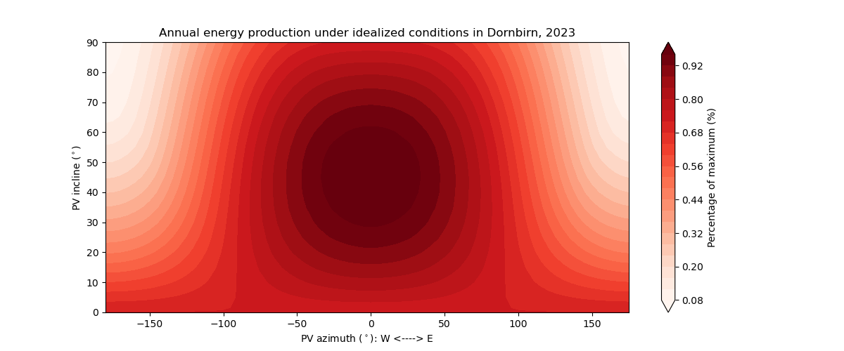
Exercise #08-01: Grid search
A grid search involves systematically searching through a predefined set of parameters to find the best parameter configuration for a specific question or model.
We aim to determine how the azimuth and incline of a PV module impact its energy production. Once again, we can utilize our existing solar module to address this question under idealized conditions and simplified assumptions.
We will perform the grid search by calling a function that does all the computations for us. In the following, I define that function and within the function body I have left you an opportunity for exercise. This task is not essential to continue with the remaining tasks. Do not get hung up here. Tip: Use the method pd.Series.diff() and the timedelta method .dt.total_seconds() to compute the time sampling in hours. If the time sampling is not equal between all time steps, raise an error.
def comp_energy_produced(iswr0, beta, pvazimuth, elevangle, azimuth, datetime = None, efficiency=0.2, area=1):
    """
    Calculate the energy produced by a PV module based on solar irradiance data.

    Parameters
    ----------
    iswr0 (pandas.Series): Solar irradiance data onto horizontal surface.
    beta (float): Incline angle of the PV module (in degrees).
    pvazimuth (float): Azimuth angle of the PV module (in degrees, 0 in the south).
    elevangle (array-like): Elevation angle of the sun (in degrees).
    azimuth (array-like): Azimuth angle of the sun (in degrees, 0 in the south).
    datetime (pandas.Series or None, optional): Timestamps associated with the irradiance data. If None,
        the function assumes regular time intervals based on the index of 'iswr0'.
    efficiency (float, optional): Efficiency of the photovoltaic system (default is 0.2).
    area (float, optional): Area of the PV module (default is 1).

    Returns
    -------
    float: Total energy produced by the photovoltaic system (in Wh).

    If 'datetime' is not provided, the function assumes regular time intervals based on the index of 'iswr0'.
    The function raises a ValueError if the time intervals are irregular.
    """

    if datetime is None:
        datetime = iswr0.index.to_series()

    # Retrieve unique time sampling dt in (hours)
    delta = datetime.diff()
    dt = delta.dt.total_seconds()/3600
    dt = dt[dt.notna()].unique()
    if (len(dt) > 1):
        raise ValueError("Irregular time sampling is not allowed")

    # Calculate iswr onto inclined PV module
    iswr_beta = solar.comp_irradiance_incline(iswr0,
                                              solar.comp_cos_incidenceangle(elevangle, azimuth, beta, pvazimuth),
                                              elevangle)
    # Calculate generated power and energy
    power = iswr_beta * area * efficiency
    energy = power.sum() * dt

    return energy[0]
Finally, you can perform the grid search:
alpha_pv = np.arange(-180, 180, 5)
beta_pv = np.arange(0, 95, 5)

APV, BPV = np.meshgrid(alpha_pv, beta_pv)
Z = np.full(APV.shape, np.nan)
for i, _ in enumerate(alpha_pv):
for j, _ in enumerate(beta_pv):
# print(i, j, APV[j, i], BPV[j, i])
Z[j, i] = comp_energy_produced(sdo['iswr_clearsky'], BPV[j, i], APV[j, i], sdo['h'], sdo['alpha'])
i_max = np.argmax(Z[~np.isnan(Z)])
Z_max = np.max(Z[~np.isnan(Z)])
Z = Z/Z_maxprint(f"Optimal PV position: azimuth {APV[np.unravel_index(i_max, APV.shape)]}, incline {BPV[np.unravel_index(i_max, APV.shape)]}")Optimal PV position: azimuth -5, incline 45f, ax = plt.subplots(figsize=(12, 5))
cf = ax.contourf(alpha_pv, beta_pv, Z, levels=30, cmap='Reds', extend='both')
cbar = f.colorbar(cf)
ax.scatter(APV[np.unravel_index(i_max, APV.shape)], BPV[np.unravel_index(i_max, APV.shape)], color='black')
cbar.set_label("Percentage of maximum (%)")
ax.set_ylabel(r"PV incline ($^\circ$)")
ax.set_xlabel(r"PV azimuth ($^\circ$): W <----> E")
ax.set_title("Annual energy production under idealized conditions in Dornbirn, 2023")
# plt.savefig("contourplot.png")Text(0.5, 1.0, 'Annual energy production under idealized conditions in Dornbirn, 2023')