import pandas as pd
import matplotlib.pyplot as pltInteractive exercise
Unit 07
#07-01: Summary stats
- Using the
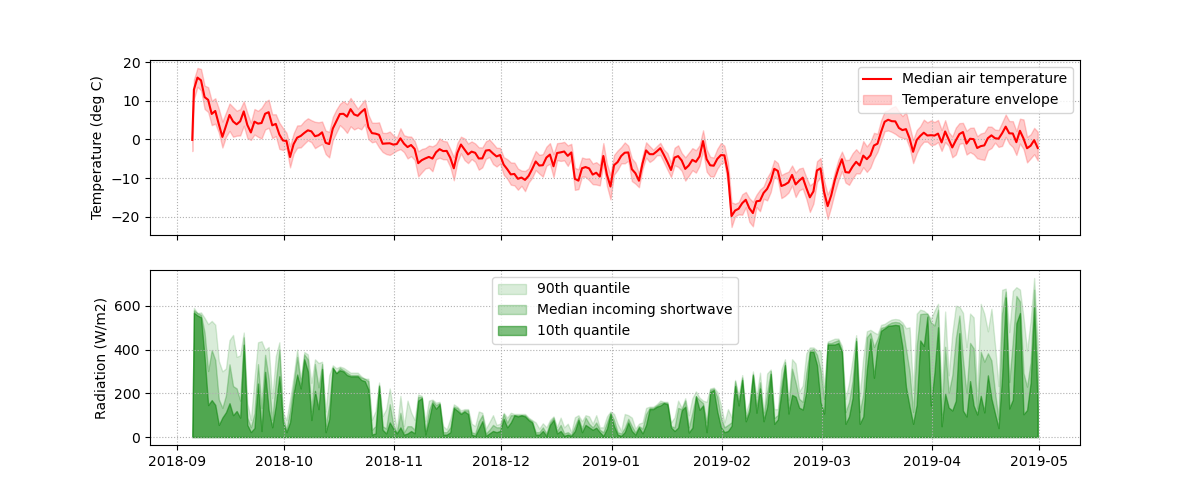
WX19data frame (see Assignment #6), compute which station has the maximum total irradiance (i.e., total incoming shortwave radiation). - Create a plot as similar as possible to the following plot.
Tip
- You should be able to compute the total irradiance for each station based on all the tips you got up until here. The step from the total irradiance at each station to getting the
station_idwith the maximum total irradiance is a bit confusing and tricky. Don’t get hung up here. - If you made it to here, you can create the figure no problem! Look into options to
plt.subplots(), the axes method.fill_between(), and control the transparency of the shaded areas with thealphaargument to your plot methods.
Solution
Notebook
Download the notebook: 07_tasks_solved.ipynb
#07-01: Summary stats
- Using the
WX19data frame, compute which station has the maximum total incoming shortwave radiation. - Create a plot as similar as possible to the following plot.
WX19 = pd.read_csv("../06_files/WX19.csv", sep=",", parse_dates=["datetime"])
WX19| datetime | station_id | ta | iswr | |
|---|---|---|---|---|
| 0 | 2018-09-05 06:00:00 | VIR075905 | -2.03788 | 0.000 |
| 1 | 2018-09-05 17:00:00 | VIR075905 | 11.10640 | 579.437 |
| 2 | 2018-09-06 17:00:00 | VIR075905 | 14.04840 | 577.724 |
| 3 | 2018-09-07 17:00:00 | VIR075905 | 13.94120 | 558.580 |
| 4 | 2018-09-08 17:00:00 | VIR075905 | 9.57504 | 511.112 |
| ... | ... | ... | ... | ... |
| 56877 | 2019-04-26 17:00:00 | VIR088016 | 1.82977 | 614.784 |
| 56878 | 2019-04-27 17:00:00 | VIR088016 | -4.01148 | 324.892 |
| 56879 | 2019-04-28 17:00:00 | VIR088016 | -2.11787 | 517.290 |
| 56880 | 2019-04-29 17:00:00 | VIR088016 | -1.73154 | 700.392 |
| 56881 | 2019-04-30 17:00:00 | VIR088016 | -3.46323 | 338.852 |
56882 rows × 4 columns
iswr_tot = WX19[["iswr", "station_id"]].groupby("station_id").sum()
iswr_tot.index[iswr_tot.values.argmax()]'VIR078109'WX19_grouped_ta = WX19[["datetime", "ta"]].groupby("datetime")
ta_lower = WX19_grouped_ta.quantile(0.1)
ta_upper = WX19_grouped_ta.quantile(0.9)
ta_median = WX19_grouped_ta.median()
WX19_grouped_iswr = WX19[["datetime", "iswr"]].groupby("datetime")
iswr_lower = WX19_grouped_iswr.quantile(0.1)
iswr_upper = WX19_grouped_iswr.quantile(0.9)
iswr_median = WX19_grouped_iswr.median()# # Loop example:
# ta_lower = np.full(WX19['datetime'].unique().shape, np.nan)
# ta_upper = np.full(WX19['datetime'].unique().shape, np.nan)
# ta_median = np.full(WX19['datetime'].unique().shape, np.nan)
# ta_dt = WX19['datetime'].unique()
# for i, dt in enumerate(ta_dt):
# ta_lower[i] = WX19.loc[WX19['datetime'] == dt, 'ta'].quantile(0.1)
# ta_upper[i] = WX19.loc[WX19['datetime'] == dt, 'ta'].quantile(0.9)
# ta_median[i] = WX19.loc[WX19['datetime'] == dt, 'ta'].median()fig, (ax1, ax2) = plt.subplots(figsize=(12, 5), nrows=2, sharex=True)
ax1.plot(ta_median, color="red")
ax1.fill_between(ta_lower.index, ta_lower["ta"], ta_upper["ta"], color="red", alpha=0.2)
ax1.legend(["Median air temperature", "Temperature envelope"])
ax1.set_ylabel("Temperature (deg C)")
ax1.grid(linestyle=":")
ax2.fill_between(iswr_lower.index, 0, iswr_upper["iswr"], color="green", alpha=0.15)
ax2.fill_between(iswr_lower.index, 0, iswr_median["iswr"], color="green", alpha=0.25)
ax2.fill_between(iswr_lower.index, 0, iswr_lower["iswr"], color="green", alpha=0.5)
ax2.legend(["90th quantile", "Median incoming shortwave", "10th quantile"], loc="upper center")
ax2.set_ylabel("Radiation (W/m2)")
ax2.grid(linestyle=":")
# fig.savefig('twopanel_pretty.png')