import pandas as pd
import matplotlib.pyplot as plt#07-01: Summary stats
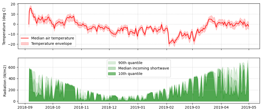
- Using the
WX19data frame, compute which station has the maximum total incoming shortwave radiation. - Create a plot as similar as possible to the following plot.
In [1]:
In [2]:
WX19 = pd.read_csv("../06_files/WX19.csv", sep=",", parse_dates=["datetime"])
WX19| datetime | station_id | ta | iswr | |
|---|---|---|---|---|
| 0 | 2018-09-05 06:00:00 | VIR075905 | -2.03788 | 0.000 |
| 1 | 2018-09-05 17:00:00 | VIR075905 | 11.10640 | 579.437 |
| 2 | 2018-09-06 17:00:00 | VIR075905 | 14.04840 | 577.724 |
| 3 | 2018-09-07 17:00:00 | VIR075905 | 13.94120 | 558.580 |
| 4 | 2018-09-08 17:00:00 | VIR075905 | 9.57504 | 511.112 |
| ... | ... | ... | ... | ... |
| 56877 | 2019-04-26 17:00:00 | VIR088016 | 1.82977 | 614.784 |
| 56878 | 2019-04-27 17:00:00 | VIR088016 | -4.01148 | 324.892 |
| 56879 | 2019-04-28 17:00:00 | VIR088016 | -2.11787 | 517.290 |
| 56880 | 2019-04-29 17:00:00 | VIR088016 | -1.73154 | 700.392 |
| 56881 | 2019-04-30 17:00:00 | VIR088016 | -3.46323 | 338.852 |
56882 rows × 4 columns
In [3]:
iswr_tot = WX19[["iswr", "station_id"]].groupby("station_id").sum()
iswr_tot.index[iswr_tot.values.argmax()]'VIR078109'In [4]:
WX19_grouped_ta = WX19[["datetime", "ta"]].groupby("datetime")
ta_lower = WX19_grouped_ta.quantile(0.1)
ta_upper = WX19_grouped_ta.quantile(0.9)
ta_median = WX19_grouped_ta.median()

WX19_grouped_iswr = WX19[["datetime", "iswr"]].groupby("datetime")
iswr_lower = WX19_grouped_iswr.quantile(0.1)
iswr_upper = WX19_grouped_iswr.quantile(0.9)
iswr_median = WX19_grouped_iswr.median()
In [2]:
# # Loop example:
# ta_lower = np.full(WX19['datetime'].unique().shape, np.nan)
# ta_upper = np.full(WX19['datetime'].unique().shape, np.nan)
# ta_median = np.full(WX19['datetime'].unique().shape, np.nan)
# ta_dt = WX19['datetime'].unique()

# for i, dt in enumerate(ta_dt):
#     ta_lower[i] = WX19.loc[WX19['datetime'] == dt, 'ta'].quantile(0.1)
#     ta_upper[i] = WX19.loc[WX19['datetime'] == dt, 'ta'].quantile(0.9)
#     ta_median[i] = WX19.loc[WX19['datetime'] == dt, 'ta'].median()
In [5]:
fig, (ax1, ax2) = plt.subplots(figsize=(12, 5), nrows=2, sharex=True)

ax1.plot(ta_median, color="red")
ax1.fill_between(ta_lower.index, ta_lower["ta"], ta_upper["ta"], color="red", alpha=0.2)
ax1.legend(["Median air temperature", "Temperature envelope"])
ax1.set_ylabel("Temperature (deg C)")
ax1.grid(linestyle=":")

ax2.fill_between(iswr_lower.index, 0, iswr_upper["iswr"], color="green", alpha=0.15)
ax2.fill_between(iswr_lower.index, 0, iswr_median["iswr"], color="green", alpha=0.25)
ax2.fill_between(iswr_lower.index, 0, iswr_lower["iswr"], color="green", alpha=0.5)
ax2.legend(["90th quantile", "Median incoming shortwave", "10th quantile"], loc="upper center")
ax2.set_ylabel("Radiation (W/m2)")
ax2.grid(linestyle=":")
# fig.savefig('twopanel_pretty.png')