Until next week, solve the following exercise in a notebook.
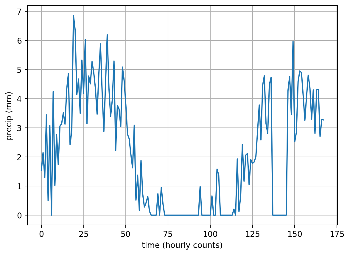
In the following exercise, you will work with synthetically created precipitation data. Let me set this ‘data set’ up for you:
import numpy as npimport matplotlib.pyplot as plt# create a "time" vector of hourly counts over 7 dayst = np.arange(24*7)# create random "outage" time and noiset_outage = np.random.randint(140, 160, 1)precip_noise = np.random.normal(1.5, 1, t.size)# create a precipitation pattern with a sine wave and superposed noiseprecip =3*np.sin(t/(6*np.pi)) + precip_noise# set all negative precip to zero and create "precipitation gauge outage"precip[precip <0] =0precip[(t > t_outage-5) & (t < t_outage+5)] =0
The previous code cell generated what I refer to as the “time” vector t for now. It symbolizes time by counting the hours of one week (=24*7 hours). It also generates a synthetic precipitation measurement from a rain gauge by combining a sine wave with random noise. Unfortunately, our rain gauge experienced a problem, which caused the measurement to be unrealiable for a short time.
Make sure you understand what the previous code cells do, before you jump to the actual exercises.
Rewrite my vectorized statement precip[(t > 150) & (t < 160)] = 0 in a for loop
Calculate the total precipitation sum at each day (i.e., Day 1 goes from 0–23) and store it in a vector precip_total. Then, plot each daily precipitation sum at noon each day with the time vector t_noon = np.arange(12, 7*24, 24). Add your result to the plot above using black circles.
Tip for Question 2
Think along the lines of iterating over the indices and elements of t_noon to compute the relevant element of precip_total from the relevant elements of precip. It might be a bit easier to get the indices right, when you actually iterate over yet a new time vector t_midnight, which is the analogon to t_noon.
Calculate the moving average of precip using a 3h time window. Implement the moving average with a for loop. Basically, at each iteration i the moving average equals the sum of precip elements from the time step before to the time step after (i.e., precip[i-1], precip[i], precip[i+1]). You will therefore not be able to compute moving averages for the first and last elements of precip. When you’re done, add the moving average to the plot.
Code a function that computes the start times of storms based on hourly precipitation data. Your algorithm should be based on the following assumptions:
We define the start time of a storm as the last hour with zero precip, one hour prior should also be precip-free, and one hour later should have non-zero precip. The first and last hours of our data set can therefore not be start times of a storm.
Implement one function that solves the challenge with a for loop, and then a second function that solves the challenges with a vectorized solution.
The functions should return lists.
Tips: use np.isclose() to check whether your floats are 0. For the vectorized approach, apply array slicing to create three slighty shifted arrays. Once you have these, you can come up with a logical expression that satisfies our defined rules.
How long did you take for each of the implementations? You get what I meant when I said vectorization can take up a bit of coding time..
Analogously, code a function that detects the start and end times of rain gauge outages based on the following assumptions:
We assume a rain gauge outage, when the precip is zero for more than three hours and when the precip drops and increases rapidly at the start/end times of the outage, i.e., with an absolute difference of more than twice the precip standard deviation.
Analogously to above, your function should return a tuple of two lists.
Tip for Question 5
In my approach, I start out by computing the difference between precip elements using np.diff(). Then, I test where this array of differences exceeds 2 standard deviations of precip using np.where(). Then I iterate over the time intervals between the abrupt changes and test whether all precip elements during these time intervals are zero. If so, I add the relevant start and end times to the lists outage_start and outage_end, which are the return variables of the function.
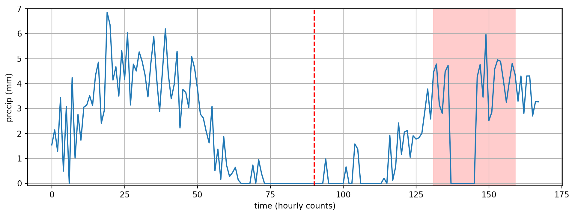
When you’re done with steps 4 and 5, edit the following code cell to adjust the plot, so that the red vertical line and red shading match the correct times based on the calculations of your functions. To do that replace the hardcoded values in the first two lines with your function calls. If you re-run the first code cell where precip is generated, you will get slightly different times. If you then run the following code cell again, you will see whether your functions pick up on the changed data set and still return the correct result. If they don’t return the correct result, try to assess whether our underlying rules and assumptions are too crude or whether there is a bug in your function.