
Grafiken
Contents
Grafiken#
Passive Grafiken: matplotlib#
Wir werden nur zwei Beispiele in diesem Abschnitt aufzeigen. Die fast unüberschaubare Vielfalt an grafischen Darstellungsmöglichkeiten mit dem Python-Paket Matplotlib finden Sie z. B. unter Matplotlib Gallery.
import numpy as np
import matplotlib.pyplot as plt
# Durch den Import des seaborn Paketes wird die Default-Darstellung von Abbildungen geändert:
import seaborn as sns
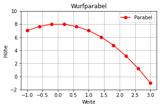
Beispiel 1: 2D-Plot
Wir plotten einen Vektor x gegen einen Vektor y:
x = np.linspace(-1, 3, num = 11)
x
array([-1. , -0.6, -0.2, 0.2, 0.6, 1. , 1.4, 1.8, 2.2, 2.6, 3. ])
# Typ des Objekts x:
type(x)
numpy.ndarray
%whos
Variable   Type       Data/Info
-------------------------------
np         module     <module 'numpy' from '/us<...>kages/numpy/__init__.py'>
plt        module     <module 'matplotlib.pyplo<...>es/matplotlib/pyplot.py'>
sns        module     <module 'seaborn' from '/<...>ges/seaborn/__init__.py'>
x          ndarray    11: 11 elems, type `float64`, 88 bytes
y = -x**2 + 8
plt.figure(figsize=(5,3))
plt.plot(x, y, 'o-r', label='Parabel')
plt.xlabel('Weite')
plt.ylabel('Höhe')
plt.ylim(-2, 10)
plt.title('Wurfparabel')
plt.legend(numpoints=1, loc='best')
plt.grid(True)

plt.savefig('abbildungen/Wurfparabel.pdf')
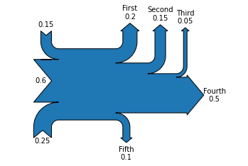
Beispiel 2: Sankey-Diagramm
Nach dem Import der Sankey Funktion erstellen wir ein Sankey-Diagramm.
from matplotlib.sankey import Sankey
fig = plt.figure(figsize=(6,4))
ax = fig.add_subplot(1,1,1)
plt.axis('off')
Sankey(flows=[0.25, 0.15, 0.60, -0.20, -0.15, -0.05, -0.50, -0.10], ax = ax,
       labels=['', '', '', 'First', 'Second', 'Third', 'Fourth', 'Fifth'],
       orientations=[-1, 1, 0, 1, 1, 1, 0, -1]).finish();

plt.savefig('abbildungen/Sankey.pdf')
Interaktive Grafiken: ipywidgets#
Link: ipywidgets.readthedocs.io/en/stable/
from ipywidgets import interact
x = np.linspace(-2, 2, num= 100)

def my_f(k):
    y = k*x
    plt.plot(x, y)
    plt.ylim((-2, 2))
    plt.xlim((-2, 2))
    plt.grid(True)
    plt.show()

interact(my_f, k=(-1, 1, 0.1));