Pandas: Visualization
Contents
Pandas: Visualization#
For more cf. Pandas Chart Visualization.
import pandas as pd
import numpy as np
import matplotlib.pyplot as plt
Plotting Features#
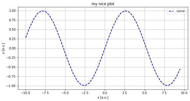
plt.figure(figsize=(10,5))

x = np.arange(start =-10, stop = 10, step=0.5)
y = np.sin(.6*x)

plt.plot(x, y, '--b', linewidth=2, label='curve')

plt.title('my nice plot')
plt.xlabel('x [a.u.]')
plt.ylabel('y [a.u.]')
plt.legend(loc='best', numpoints=3)
plt.grid()

plt.savefig('abbildungen/my_plot.pdf')
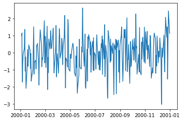
Random Walk with Series#
dates = pd.date_range('2000-01-01', '2001-01-01', freq='B')
ts = pd.Series(np.random.randn(len(dates)), index=dates)
ts.head()
2000-01-03    0.986342
2000-01-04    1.148306
2000-01-05   -1.725368
2000-01-06   -0.633592
2000-01-07   -0.086018
Freq: B, dtype: float64
plt.plot(ts);
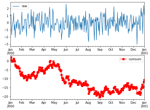
This can be plotted nicer using pandas plot method:
plt.figure(figsize=(8,6))
plt.grid()
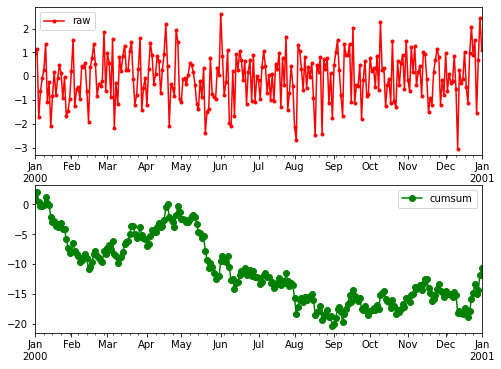
plt.subplot(2,1,1)
ts.plot(label='raw')
plt.legend()
plt.subplot(2,1,2)
ts.cumsum().plot(style='s-r', label='cumsum')
plt.legend();
df = pd.DataFrame({'raw':ts, 'cumsum':ts.cumsum()}, columns=['raw','cumsum'])
df.tail()
| raw | cumsum | |
|---|---|---|
| 2000-12-26 | 1.507907 | -13.362592 |
| 2000-12-27 | -1.551516 | -14.914108 |
| 2000-12-28 | 0.690827 | -14.223281 |
| 2000-12-29 | 2.444438 | -11.778843 |
| 2001-01-01 | 1.119174 | -10.659669 |
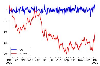
df.plot(figsize=(8,6), subplots=True, style=['.-r','o-g'], sharex=False);
df.plot(style=['b','r']);
Bar Plots#
Bar Plots of Series:
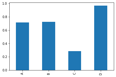
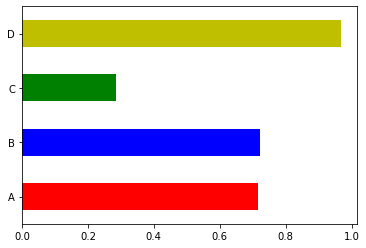
s = pd.Series(np.random.rand(4), index=['A','B','C','D'])
s
A    0.716410
B    0.723100
C    0.286061
D    0.967280
dtype: float64
s.plot(kind='bar');
s.plot(kind='barh', color=['r','b','g','y']);
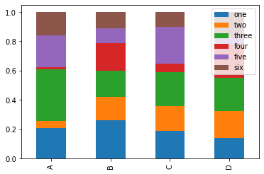
*Bar Plots of Data Frames:
df = pd.DataFrame(np.random.rand(6,4),
                  index=['one','two','three','four','five','six'],
                  columns=['A','B','C','D'])
df
| A | B | C | D | |
|---|---|---|---|---|
| one | 0.547516 | 0.919091 | 0.749656 | 0.489452 |
| two | 0.126288 | 0.566826 | 0.665307 | 0.647030 |
| three | 0.935753 | 0.633396 | 0.916266 | 0.805464 |
| four | 0.038519 | 0.676239 | 0.241718 | 0.808550 |
| five | 0.578486 | 0.355255 | 0.991703 | 0.161532 |
| six | 0.424310 | 0.396545 | 0.403273 | 0.621927 |
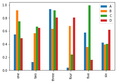
df.plot(kind='bar');
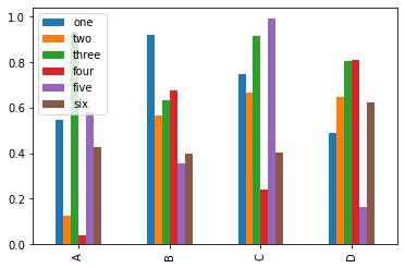
df.T.plot(kind='bar');
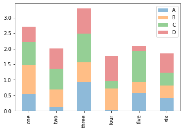
df.plot(kind='bar', stacked=True, alpha=0.5);
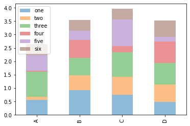
df.T.plot(kind='bar', stacked=True, alpha=0.5);
df2 = df/df.sum()
df2.T.plot(kind='bar', stacked=True, xlim= (0,6));
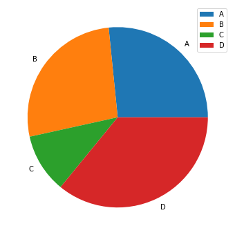
Pie Plots#
plt.figure(figsize=(6,6))
plt.pie(s, labels=s.index)
plt.legend();
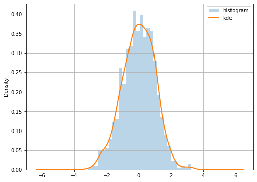
Histograms and Kernel Density Estimate#
s = pd.Series(np.random.randn(1000))

plt.figure(figsize=(8,6))
s.hist(bins=30, density=True, alpha=0.3, label='histogram')
s.plot(kind='kde', label='kde', linewidth=2)
plt.grid(True)
plt.legend();
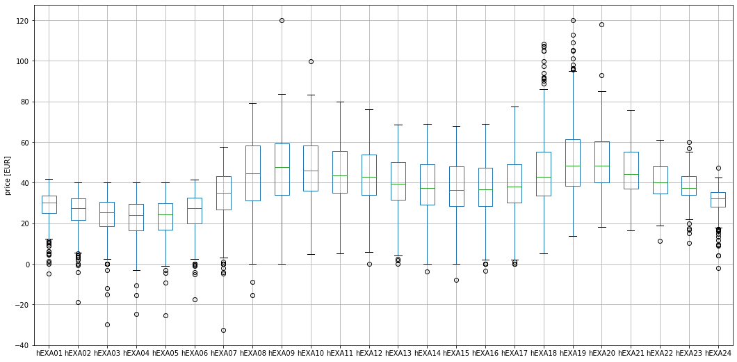
Box and Scatter Plots#
http://de.wikipedia.org/wiki/Boxplot
df = pd.read_excel('daten/dshistory2013.xls',sheet_name='Price (EUR)',skiprows=1,index_col=0)
df.head()
| hEXA01 | hEXA02 | hEXA03 | hEXA04 | hEXA05 | hEXA06 | hEXA07 | hEXA08 | hEXA09 | hEXA10 | ... | bEXAoff1\n(01-08) | bEXAoff2\n(21-24) | bEXAdream (01-06) | bEXAlunch (11-14) | bEXAteatime (17-20) | bEXAmoon\n(01-04) | bEXAsun\n(05-08) | bEXAearlyt\n(09-10) | bEXAlatet\n(15-16) | bEXAwakeup\n(07-08) | |
|---|---|---|---|---|---|---|---|---|---|---|---|---|---|---|---|---|---|---|---|---|---|
| Delivery Date | |||||||||||||||||||||
| 2013-12-31 | 20.00 | 17.26 | 15.66 | 12.00 | 12.00 | 17.61 | 22.96 | 27.04 | 33.05 | 36.15 | ... | 18.07 | 27.64 | 15.76 | 32.06 | 37.40 | 16.23 | 19.90 | 34.60 | 32.00 | 25.00 |
| 2013-12-30 | 19.67 | 13.5 | 11.44 | 11.00 | 12.63 | 18.75 | 30.00 | 33.90 | 35.76 | 37.80 | ... | 18.86 | 34.53 | 14.50 | 36.28 | 43.43 | 13.90 | 23.82 | 36.78 | 34.33 | 31.95 |
| 2013-12-29 | 16.99 | 10.56 | 7.48 | 7.13 | 7.30 | 9.65 | 14.35 | 17.49 | 19.59 | 25.55 | ... | 11.37 | 36.30 | 9.85 | 31.53 | 40.95 | 10.54 | 12.20 | 22.57 | 29.43 | 15.92 |
| 2013-12-28 | 9.00 | 5.6 | 2.39 | 3.20 | 3.77 | 7.54 | 11.58 | 18.93 | 26.81 | 30.51 | ... | 7.75 | 32.26 | 5.25 | 34.51 | 44.78 | 5.05 | 10.46 | 28.66 | 35.26 | 15.26 |
| 2013-12-27 | 20.90 | 20.03 | 15.87 | 14.93 | 17.58 | 21.13 | 23.43 | 28.44 | 32.87 | 33.93 | ... | 20.29 | 17.66 | 18.41 | 32.62 | 33.50 | 17.93 | 22.65 | 33.40 | 29.92 | 25.94 |
5 rows × 38 columns
Find non-numeric values: cf. stackoverflow
The applymap method applies a function to each element in the data frame.
df.applymap(np.isreal).head()
| hEXA01 | hEXA02 | hEXA03 | hEXA04 | hEXA05 | hEXA06 | hEXA07 | hEXA08 | hEXA09 | hEXA10 | ... | bEXAoff1\n(01-08) | bEXAoff2\n(21-24) | bEXAdream (01-06) | bEXAlunch (11-14) | bEXAteatime (17-20) | bEXAmoon\n(01-04) | bEXAsun\n(05-08) | bEXAearlyt\n(09-10) | bEXAlatet\n(15-16) | bEXAwakeup\n(07-08) | |
|---|---|---|---|---|---|---|---|---|---|---|---|---|---|---|---|---|---|---|---|---|---|
| Delivery Date | |||||||||||||||||||||
| 2013-12-31 | True | True | True | True | True | True | True | True | True | True | ... | True | True | True | True | True | True | True | True | True | True |
| 2013-12-30 | True | True | True | True | True | True | True | True | True | True | ... | True | True | True | True | True | True | True | True | True | True |
| 2013-12-29 | True | True | True | True | True | True | True | True | True | True | ... | True | True | True | True | True | True | True | True | True | True |
| 2013-12-28 | True | True | True | True | True | True | True | True | True | True | ... | True | True | True | True | True | True | True | True | True | True |
| 2013-12-27 | True | True | True | True | True | True | True | True | True | True | ... | True | True | True | True | True | True | True | True | True | True |
5 rows × 38 columns
If all in the row are True then they are all numeric:
df.applymap(np.isreal).all(1).head()
Delivery Date
2013-12-31    True
2013-12-30    True
2013-12-29    True
2013-12-28    True
2013-12-27    True
dtype: bool
Use the negation to index the data frame for those rows which have at least one non-real value:
df[~df.applymap(np.isreal).all(1)]
| hEXA01 | hEXA02 | hEXA03 | hEXA04 | hEXA05 | hEXA06 | hEXA07 | hEXA08 | hEXA09 | hEXA10 | ... | bEXAoff1\n(01-08) | bEXAoff2\n(21-24) | bEXAdream (01-06) | bEXAlunch (11-14) | bEXAteatime (17-20) | bEXAmoon\n(01-04) | bEXAsun\n(05-08) | bEXAearlyt\n(09-10) | bEXAlatet\n(15-16) | bEXAwakeup\n(07-08) | |
|---|---|---|---|---|---|---|---|---|---|---|---|---|---|---|---|---|---|---|---|---|---|
| Delivery Date | |||||||||||||||||||||
| 2013-10-27 | 12.3 | 6,74 | 4,25 | 4.0 | 0.1 | -0.2 | -0.57 | 0.98 | 6.68 | 3.98 | 9.45 | ... | 3.81 | 13.68 | 3.8 | 4.48 | 21.25 | 5.48 | 1.72 | 6.72 | -5.75 | 3.83 |
1 rows × 38 columns
df.loc['2013-10-27','hEXA02'] = 5.1
df.loc['2013-10-27','hEXA02']
5.1
Use only the first 24 columns of month data and map all values to floating point numbers.
df = df.iloc[:,:24].applymap(float)
df.columns
Index(['hEXA01', 'hEXA02', 'hEXA03', 'hEXA04', 'hEXA05', 'hEXA06', 'hEXA07',
       'hEXA08', 'hEXA09', 'hEXA10', 'hEXA11', 'hEXA12', 'hEXA13', 'hEXA14',
       'hEXA15', 'hEXA16', 'hEXA17', 'hEXA18', 'hEXA19', 'hEXA20', 'hEXA21',
       'hEXA22', 'hEXA23', 'hEXA24'],
      dtype='object')
df.boxplot(figsize=(18,9))
plt.ylabel('price [EUR]');
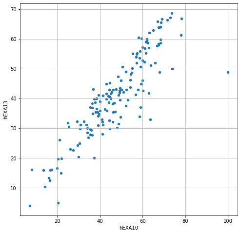
df.loc[:'2013-06-01'].plot(kind='scatter', x='hEXA10', y='hEXA13', figsize=(8,8));
plt.grid()
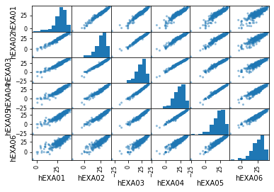
pd.plotting.scatter_matrix(df.iloc[:,:6]);
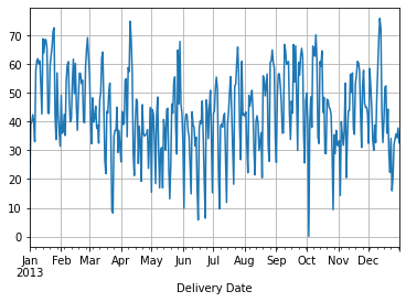
df['hEXA12'].plot();
plt.grid()
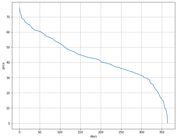
plt.figure(figsize=(10,8))
plt.plot(df['hEXA12'].sort_values(ascending=False).values)

plt.xlabel('days')
plt.ylabel('price')
plt.grid()